

Last year, AWS announced an integration between Amazon SageMaker Unified Studio and Amazon S3 general purpose buckets. This integration makes it straightforward for teams to use unstructured data stored in Amazon Simple Storage Service (Amazon S3) for machine learning (ML) and data analytics use cases.
In this post, we show how to integrate S3 general purpose buckets with Amazon SageMaker Catalog to fine-tune Llama 3.2 11B Vision Instruct for visual question answering (VQA) using Amazon SageMaker Unified Studio. For this task, we provide our large language model (LLM) with an input image and question and receive an answer. For example, asking to identify the transaction date from an itemized receipt:
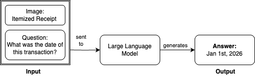
For this demonstration, we use Amazon SageMaker JumpStart to access the Llama 3.2 11B Vision Instruct model. Out of the box, this base model achieves an Average Normalized Levenshtein Similarity (ANLS) score of 85.3% on the DocVQA dataset. ANLS is a metric used to evaluate the performance of models on visual question answering tasks, which measures the similarity between the model’s predicted answer and the ground truth answer. While 85.3% demonstrates strong baseline performance, this level might not be the most efficient for tasks requiring a higher degree of accuracy and precision.
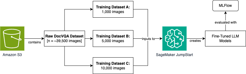
To improve model performance through fine-tuning, we’ll use the DocVQA dataset from Hugging Face. This dataset contains 39,500 rows of training data, each with an input image, a question, and a corresponding expected answer. We’ll create three fine-tuned model versions using varying dataset sizes (1,000, 5,000, and 10,000 images). We’ll then evaluate them using Amazon SageMaker fully managed serverless MLflow to track experimentation and measure accuracy improvements.
The full end-to-end data ingestion, model development, and metric evaluation process will be orchestrated using Amazon SageMaker Unified Studio. Here is the high-level process flow diagram that we’ll step through for this scenario. We’ll expand on this throughout the blog post.
To achieve this process flow, we build an architecture that performs the data ingestion, data preprocessing, model training, and evaluation using Amazon SageMaker Unified Studio. We break out each step in the following sections.
The Jupyter notebook used and referenced throughout this exercise can be found in this GitHub repository.
Prerequisites
To prepare your organization to use the new integration between Amazon SageMaker Unified Studio and Amazon S3 general purpose buckets, you must complete the following prerequisites. Note that these steps take place on an Identity Center-based domain.
- Create an AWS account.
- Create an Amazon SageMaker Unified Studio domain using quick setup.
- Create two projects within the SageMaker Unified Studio domain to model the scenario in this post: one for the data producer persona and one for the data consumer persona. The first project is used for discovering and cataloging the dataset in an Amazon S3 bucket. The second project consumes the dataset to fine-tune three iterations of our large language model. See Create a project for additional information.
- Your data consumer project must have access to a running SageMaker managed MLflow serverless application, which will be used for experimentation and evaluation purposes. For more information, see the instructions for creating a serverless MLflow application.
- An Amazon S3 bucket should be pre-populated with the raw dataset to be used for your ML development use case. In this blog post, we use the DocVQA dataset from Hugging Face for fine-tuning a visual question answering (VQA) use case.
- A service quota increase request to use p4de.24xlarge compute for training jobs. See Requesting a quota increase for more information.
Architecture
The following is the reference architecture that we build throughout this post:
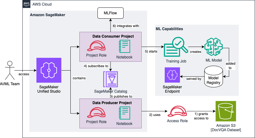
We can break the architecture diagram into a series of six high-level steps, which we’ll observe throughout the following sections:
- First, you create and configure an IAM access role that grants read permissions to a pre-existing Amazon S3 bucket containing the raw and unprocessed DocVQA dataset.
- The data producer project uses the access role to discover and add the dataset to the project catalog.
- The data producer project enriches the dataset with optional metadata and publishes it to the SageMaker Catalog.
- The data consumer project subscribes to the published dataset, making it available to the project team responsible for developing (or fine-tuning) the machine learning models.
- The data consumer project preprocesses the data and transforms it into three training datasets of varying sizes (1k, 5k, and 10k images). Each dataset is used to fine-tune our base large language model.
- We use MLflow for tracking experimentation and evaluation results of the three models against our Average Normalized Levenshtein Similarity (ANLS) success metric.
Solution walkthrough
As mentioned previously, we will opt to use the DocVQA dataset from Hugging Face for a visual question answering task. In your organization’s scenario, this raw dataset might be any unstructured data relevant to your ML use case. Examples include customer support chat logs, internal documents, product reviews, legal contracts, research papers, social media posts, email archives, sensor data, and financial transaction records.
In the prerequisite section of our Jupyter notebook, we pre-populate our Amazon S3 bucket using the Datasets API from Hugging Face:
After retrieving the dataset, we complete the prerequisite by synchronizing it to an Amazon S3 bucket. This represents the bucket depicted in the bottom-right section of our architecture diagram shown previously.
At this point, we’re ready to begin working with our data in Amazon SageMaker Unified Studio, starting with our data producer project. A project in Amazon SageMaker Unified Studio is a boundary within a domain where you can collaborate with others on a business use case. To bring Amazon S3 data into your project, you must first add access to the data and then add the data to your project. In this post, we follow the approach of using an access role to facilitate this process. See Adding Amazon S3 data for more information.
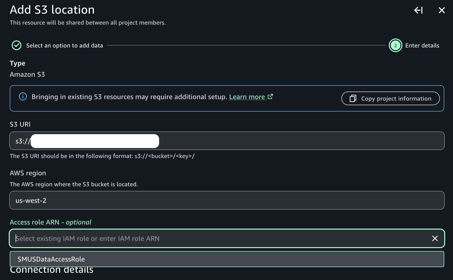
Once our access role is created following the instructions in the documentation referenced previously, we can continue with discovering and cataloging our dataset. In our data producer project, we navigate to the Data → Add data → Add S3 location:
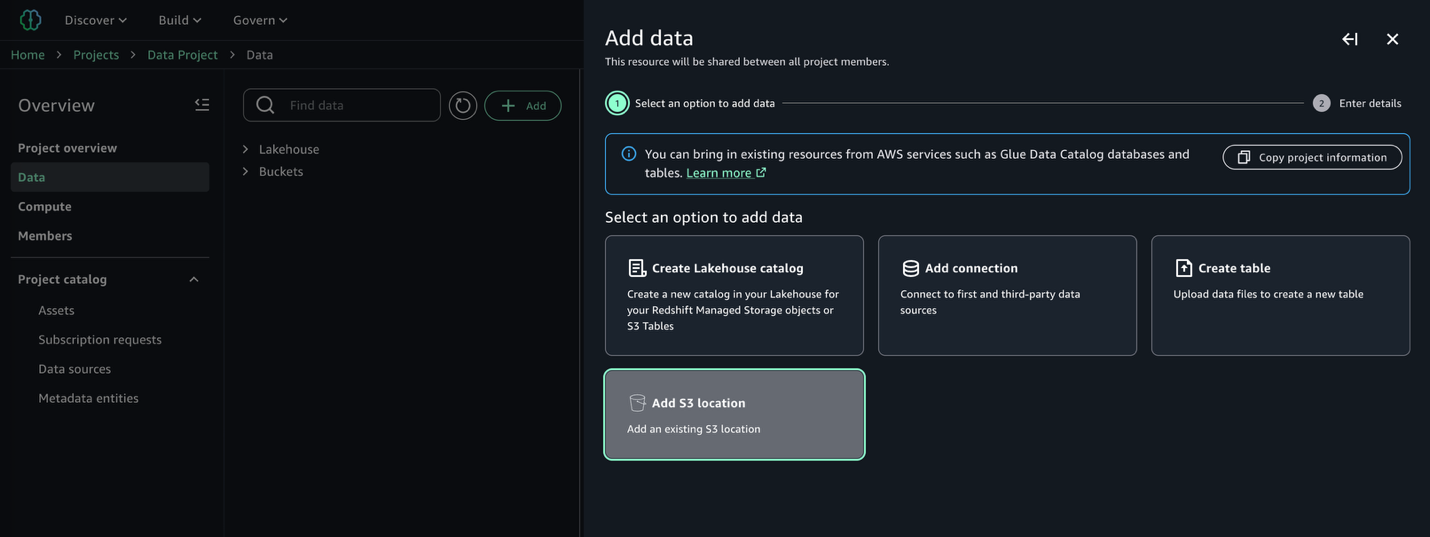
Provide the name of the Amazon S3 bucket and corresponding prefix containing our raw data, and note the presence of the access role dropdown containing the prerequisite access role previously created:
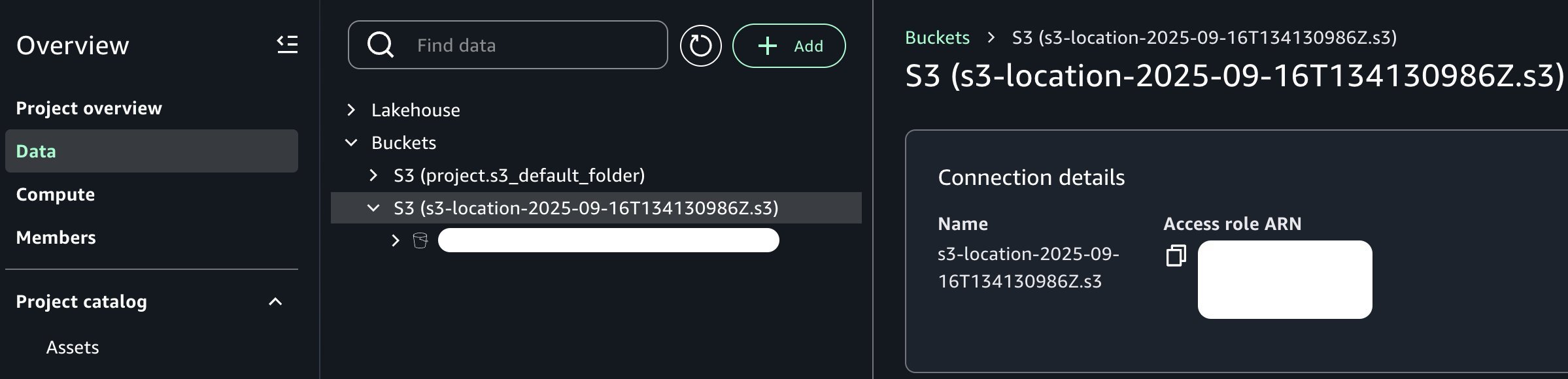
Once added, note that we can now see our new Amazon S3 bucket in the project catalog as shown in the following image:
From the perspective of our data producer persona, the dataset is now available within our project context. Depending on your organization and requirements, you might want to further enrich this data asset. For example, you can join it with additional data sources, apply business-specific transformations, implement data quality checks, or create derived features through feature engineering pipelines. However, for the purposes of this post, we’ll work with the dataset in its current form to keep our focus on the core point of integrating Amazon S3 general purpose buckets with Amazon SageMaker Unified Studio.
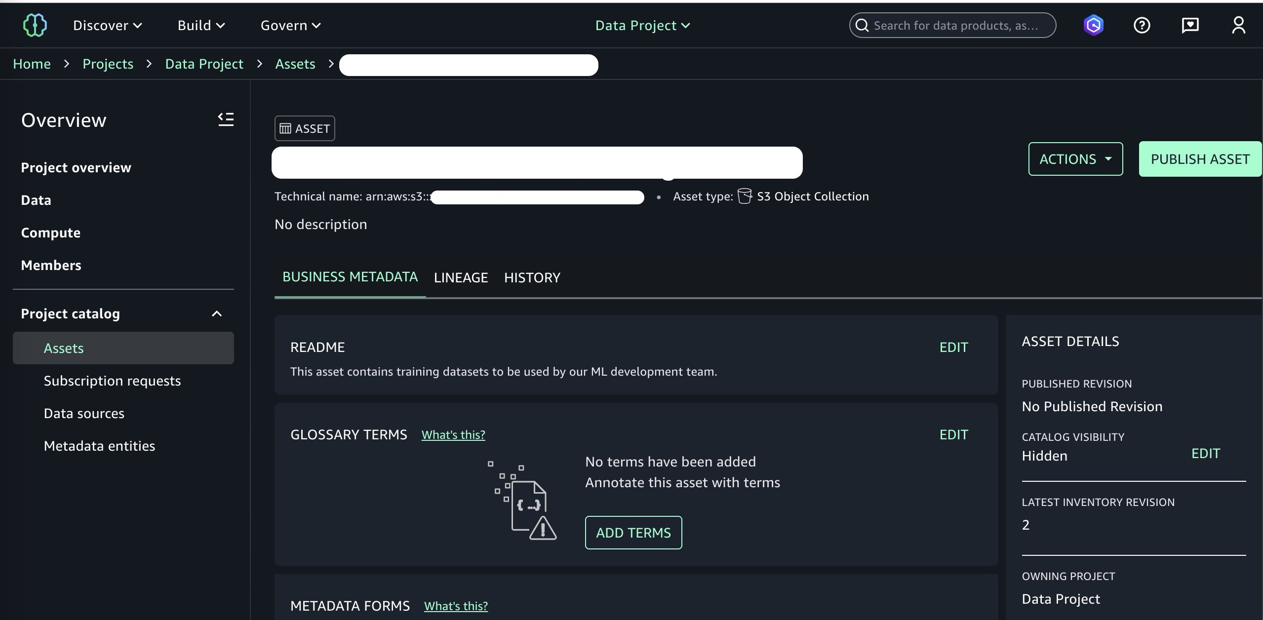
We are now ready to publish this bucket to our SageMaker Catalog. We can add optional business metadata such as a README file, glossary terms, and other data types. We add a simple README, skip other metadata fields for brevity, and continue to publishing by choosing Publish to Catalog under the Actions menu.
At this point, we’ve added the data asset to our SageMaker Catalog and it is ready to be consumed by other projects in our domain. Switching over to the perspective of our data consumer persona and selecting the consumer project, we can now subscribe to our newly published data asset. See Subscribe to a data product in Amazon SageMaker Unified Studio for more information.
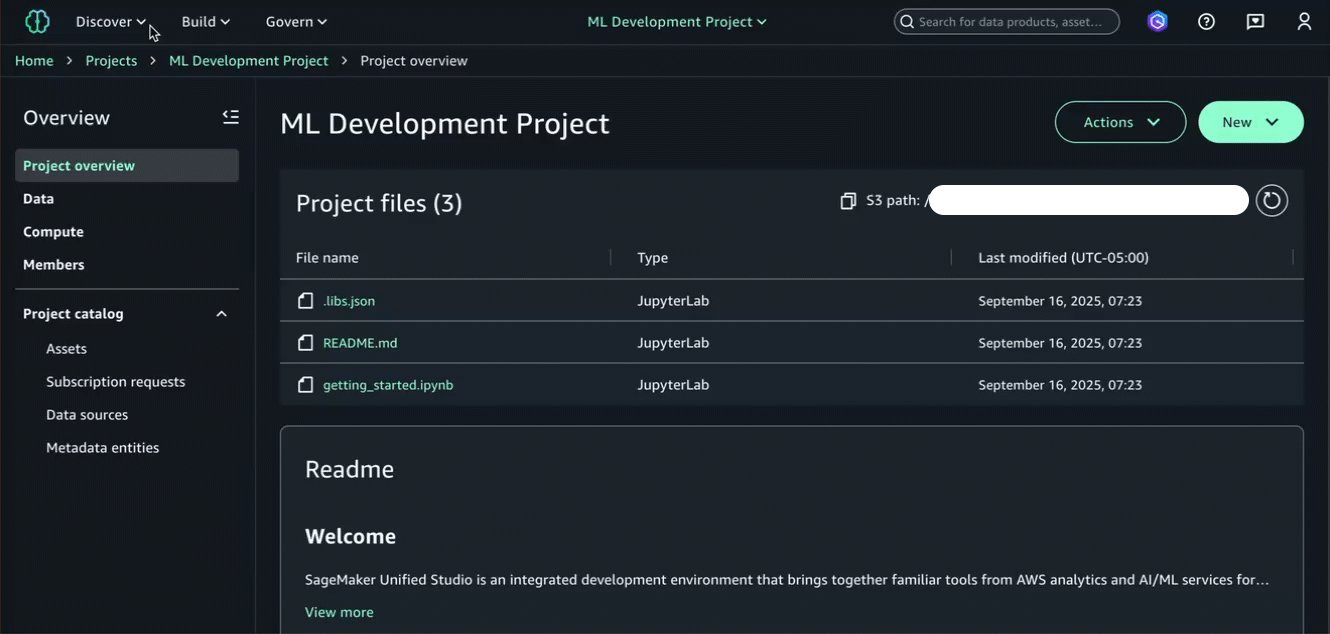
Now that we’ve subscribed to the data asset in our consumer project where we’ll build the ML model, we can begin using it within a managed JupyterLab IDE in Amazon SageMaker Unified Studio. The JupyterLab page of Amazon SageMaker Unified Studio provides a JupyterLab interactive development environment (IDE) for you to use as you perform data integration, analytics, or machine learning in your projects.
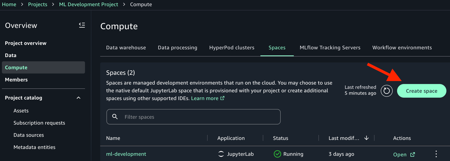
In our ML development project, navigate to the Compute → Spaces → Create space option, and choose JupyterLab in the Application (space type) menu to launch a new JupyterLab IDE.
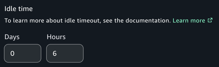
Note that some models in our example notebook can take upwards of 4 hours to train using the ml.p4de.24xlarge instance type. As a result, we recommend that you set the Idle Time to 6 hours to allow the notebook to run to completion and avoid errors. Additionally, if executing the notebook from end to end for the first time, set the space storage to 100 GB to allow for the dataset to be fully ingested during the fine-tuning process. See Creating a new space for more information.
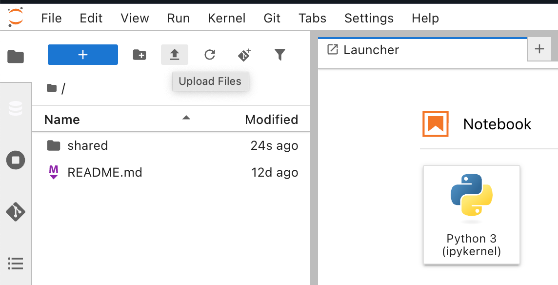
With our space created and running, we choose the Open button to launch the JupyterLab IDE. Once loaded, we upload the sample Jupyter notebook into our space using the Upload Files functionality.
Now that we’ve subscribed to the published dataset in our ML development project, we can begin the model development workflow. This involves three key steps: fetching the dataset from our bucket using Amazon S3 Access Grants, preparing it for fine-tuning, and training our models.
Grantees can access Amazon S3 data by using the AWS Command Line Interface (AWS CLI), the AWS SDKs, and the Amazon S3 REST API. Additionally, you can use the AWS Python and Java plugins to call Amazon S3 Access Grants. For brevity, we opt for the AWS CLI approach in the notebook and the following code. We also include a sample that shows the use of the Python boto3-s3-access-grants-plugin in the appendix section of the notebook for reference.
The process includes two steps: first obtaining temporary access credentials to the Amazon S3 control plane through the s3control CLI module, then using those credentials to sync the data locally. Update the AWS_ACCOUNT_ID variable with the appropriate account ID that houses your dataset.
import json

AWS_ACCOUNT_ID = "123456789" # REPLACE THIS WITH YOUR ACCOUNT ID
S3_BUCKET_NAME = "s3://MY_BUCKET_NAME/" # REPLACE THIS WITH YOUR BUCKET

# Get credentials
result = !aws s3control get-data-access --account-id {AWS_ACCOUNT_ID} --target {S3_BUCKET_NAME} --permission READ

json_response = json.loads(result.s)
creds = json_response['Credentials']

# Configure profile with cell magic
!aws configure set aws_access_key_id {creds['AccessKeyId']} --profile access-grants-consumer-access-profile
!aws configure set aws_secret_access_key {creds['SecretAccessKey']} --profile access-grants-consumer-access-profile
!aws configure set aws_session_token {creds['SessionToken']} --profile access-grants-consumer-access-profile

print("Profile configured successfully!")

!aws s3 sync {S3_BUCKET_NAME} ./ --profile access-grants-consumer-access-profile
After running the previous code and getting a successful output, we can now access the S3 bucket locally. With our raw dataset now accessible locally, we need to transform it into the format required for fine-tuning our LLM. We’ll create three datasets of varying sizes (1k, 5k, and 10k images) to evaluate how the dataset size impacts model performance.
Each training dataset contains a train and validation directory, each of which must contain an images subdirectory and accompanying metadata.jsonl file with training examples. The metadata file format includes three key/value fields per line:
With these artifacts uploaded to Amazon S3, we can now fine-tune our LLM by using SageMaker JumpStart to access the pre-trained Llama 3.2 11B Vision Instruct model. We’ll create three separate fine-tuned variants to evaluate. We’ve created a train() function to facilitate this using a parameterized approach, making this reusable for different dataset sizes:
Our training function handles several important aspects:
- Model selection: Uses the latest version of Llama 3.2 11B Vision Instruct from SageMaker JumpStart.
- Hyperparameters: The sample notebook uses the retrieve_default() API in the SageMaker SDK to automatically fetch the default hyperparameters for our model.
- Batch size: The only default hyperparameter that we change, setting to 1 per device due to the large model size and memory constraints.
- Instance type: We use a ml.p4de.24xlarge instance type for this training job and recommend that you use the same type or larger.
- MLflow integration: Automatically logs hyperparameters, job names, and training metadata for experiment tracking.
- Endpoint deployment: Automatically deploys each trained model to a SageMaker endpoint for inference.
Recall that the training process will take a few hours to complete using instance type ml.p4de.24xlarge.
Now we’ll evaluate our fine-tuned models using the Average Normalized Levenshtein Similarity (ANLS) metric. This metric evaluates text-based outputs by measuring the similarity between predicted and ground truth answers, even when there are minor errors or variations. It is particularly useful for tasks like visual question answering because it can handle slight variations in answers. See the Llama 3.2 3B model card for more information.
MLflow will track our experiments and results for straightforward comparison. Our evaluation pipeline includes several key functions for image encoding for model inference, payload formatting, ANLS calculation, and results tracking. The training_pipeline() function orchestrates the complete workflow with nested MLflow runs for better experiment organization.
After orchestrating three end-to-end executions for our three dataset sizes, we review the ANLS metric results in MLflow. Using the comparison functionality, we note the highest ANLS score of 0.902 in the docvqa-10000 model, an increase of 4.9 percentage points relative to the base model (0.902 − 0.853 = 0.049).
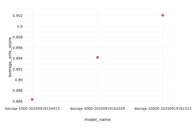
| Model | ANLS |
| docvqa-1000 | 0.886 |
| docvqa-5000 | 0.894 |
| docvqa-10000 | 0.902 |
| Base Model | 0.853 |
Clean Up
To avoid ongoing charges, delete the resources created during this walkthrough. This includes SageMaker endpoints and project resources such as the MLflow application, JupyterLab IDE, and domain.
Conclusion
Based on the preceding data, we observe a positive relationship between the size of the training dataset and ANLS in that the docvqa-10000 model had improved performance.
We used MLflow for experimentation and visualization around our success metric. Further improvements in areas such as hyperparameter tuning and data enrichment could yield even better results.
This walkthrough demonstrates how the Amazon SageMaker Unified Studio integration with S3 general purpose buckets helps streamline the path from unstructured data to production-ready ML models. Key benefits include:
- Simplified data discovery and cataloging through a unified interface
- More secure data access through S3 Access Grants without complex permission management
- Smooth collaboration between data producers and consumers across projects
- End-to-end experiment tracking with managed MLflow integration
Organizations can now use their existing S3 data assets more effectively for ML workloads while maintaining governance and security controls. The 4.9% performance improvement from base model to our improved fine-tuned variant (0.853–0.902 ANLS) validates the approach for visual question answering tasks.
For next steps, consider exploring additional dataset preprocessing techniques, experimenting with different model architectures available through SageMaker JumpStart, or scaling to larger datasets as your use case demands.
- Getting Started with Amazon SageMaker JumpStart
- Data transformation workloads with SageMaker Processing
The solution code used for this blog post can be found in this GitHub repository.


