Accelerating LLM inference with post-training weight and activation using AWQ and GPTQ on Amazon SageMaker AI

Foundation models (FMs) and large language models (LLMs) have been rapidly scaling, often doubling in parameter count within months, leading to significant improvements in language understanding and generative capabilities. This rapid growth comes with steep costs: inference now requires enormous memory capacity, high-performance GPUs, and substantial energy consumption. This trend is evident in the open source space. In 2023, TII-UAE released Falcon 180B, the largest open model at the time. Meta surpassed that in 2024 with Llama 3.1, a 405B dense model. As of mid-2025, the largest publicly available model is DeepSeek (V3 – Instruct variant, R1 – Reasoning variant), a mixture of experts (MoE) architecture with 671 billion total parameters—of which 37 billion are active per token. These models deliver state-of-the-art performance across a wide range of tasks, including multi-modal search, code generation, summarization, idea generation, logical reasoning, and even PhD-level problem solving. Despite their value, deploying such models in real-world applications remains largely impractical because of their size, cost, and infrastructure requirements.

We often rely on the intelligence of large models for mission-critical applications such as customer-facing assistants, medical research, or enterprise agents, where hallucinations can lead to serious consequences. However, deploying models with over 100 billion parameters at scale is technically challenging—these models require significant GPU resources and memory bandwidth, making it difficult to spin up or scale down instances quickly in response to fluctuating user demand. As a result, scaling to thousands of users quickly becomes cost-prohibitive, because the high-performance infrastructure requirements make the return on investment (ROI) difficult to justify. Post-training quantization (PTQ) offers a practical alternative; by converting 16- or 32-bit weights and activations into lower-precision 8- or 4-bit integers after training, PTQ can shrink model size by 2–8 times, reduce memory bandwidth requirements, and speed up matrix operations, all without the need for retraining, making it suitable for deploying large models more efficiently. For example, the base DeepSeek-V3 model requires an ml.p5e.48xlarge instance (with 1128 GB H100 GPU memory) for inference, while its quantized variant (QuixiAI/DeepSeek-V3-0324-AWQ) can run on smaller instances such as ml.p5.48xlarge (with 640 GB H100 GPU memory) or even ml.p4de.24xlarge (with 640 GB A100 GPU memory). This efficiency is achieved by applying low-bit quantization to less influential weight channels, while preserving or rescaling the channels that have the greatest impact on activation responses, and keeping activations in full precision—dramatically reducing peak memory usage.

Quantized models are made possible by contributions from the developer community—including projects like Unsloth AI and QuixiAI (formerly: Cognitive Computations)—that invest significant time and resources into optimizing LLMs for efficient inference. These quantized models can be seamlessly deployed on Amazon SageMaker AI using a few lines of code. Amazon SageMaker Inference provides a fully managed service for hosting machine learning, deep learning, and large language or vision models at scale in a cost-effective and production-ready manner. In this post, we explore why quantization matters—how it enables lower-cost inference, supports deployment on resource-constrained hardware, and reduces both the financial and environmental impact of modern LLMs, while preserving most of their original performance. We also take a deep dive into the principles behind PTQ and demonstrate how to quantize the model of your choice and deploy it on Amazon SageMaker.

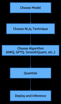
The steps are:

1. Choose model
2. Choose W_xA_y technique (W_xA_y here implies weights and activations, which will be discussed in depth later in this post)
3. Choose algorithm (AWQ, GPTQ, SmoothQuant, and so on)
4. Quantize
5. Deploy and inference

To illustrate this workflow and help visualize the process, we’ve included the following flow diagram.

Prerequisites

To run the example notebooks, you need an AWS account with an AWS Identity and Access Management (IAM) role with permissions to manage resources created. For more information, see Create an AWS account.

If this is your first time working with Amazon SageMaker Studio, you first need to create a SageMaker domain.

By default, the model runs in a shared AWS managed virtual private cloud (VPC) with internet access. To enhance security and control access, you should explicitly configure a private VPC with appropriate security groups and IAM policies based on your requirements.

Amazon SageMaker AI provides enterprise-grade security features to help keep your data and applications secure and private. We don’t share your data with model providers, providing you full control over your data. This applies to all models—both proprietary and publicly available, including DeepSeek-R1 on SageMaker. For more information, see Configure security in Amazon SageMaker AI.

As a best practice, it’s always recommended to deploy your LLM’s endpoints inside your VPC and behind a private subnet without internet gateways and preferably with no egress. Ingress from the internet should also be blocked to minimize security risks.

In this post, we use LiteLLM Python SDK to standardize and abstract access to Amazon SageMaker real-time endpoints and LLMPerf tool for evaluation of performance of our quantized models. See Installation in the LLMPerf GitHub repo for setup instructions.

Weights and activation techniques (WₓAᵧ)

As the scale of LLMs continues to grow, deploying them efficiently becomes less about raw performance and more about finding the right balance between speed, cost, and accuracy. In real-world scenarios, quantization starts with three core considerations:

• The size of the model you need to host
• The cost or target hardware available for inference
• The acceptable trade-off between accuracy and inference speed

Understanding how these factors shape quantization choices is key to making LLMs viable in production environments. We’ll explore how post-training quantization techniques like AWQ and generative pre-trained transformers quantization (GPTQ) help navigate these constraints and make state-of-the-art models deployable at scale.

Weights and activation: A deep dive

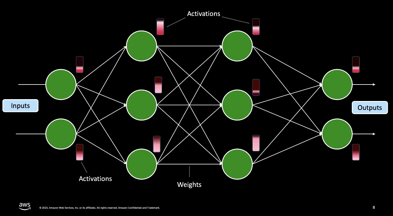
In neural networks, weights are the static, learned parameters saved in the model—think of them as the fixed coefficients that shape how inputs are combined—while activations are the dynamic values produced at each layer when you run data through the network, representing the response of each neuron to its inputs. The preceding figure illustrates weights and activations in a model flow. We capture their respective precisions with the shorthand WₓAᵧ, where Wₓ is the bit-width for weights (for example, 4-bit or 8-bit) and Aᵧ is the bit-width for activations (for example, 8-bit or 16-bit). For example, W4A16 means weights are stored as 4-bit integers (often with per-channel, symmetric or asymmetric scaling) while activations remain in 16-bit floating point. This notation tells you which parts of the model are compressed and by how much, helping you balance memory use, compute speed, and accuracy.

W4A16 (or W4A16_symmetric)

W4A16 refers to 4-bit precision for weights and 16-bit for activations, using a symmetric quantization for weights. Symmetric quantization means the quantizer’s range is centered around zero (the absolute minimum and maximum of the weight distribution are set to be equal in magnitude). Using 4-bit integer weights yields an 8-times reduction in weight memory compared to FP32 (or 4 times compared to FP16), which is very attractive for deployment. However, with only 16 quantization levels (−8 to +7 for a 4-bit signed integer, in a symmetric scheme), the model is prone to quantization error. If the weight distribution isn’t perfectly zero-centered (for example, if weights have a slight bias or a few large outliers), a symmetric quantizer might waste range on one side and not have enough resolution where the bulk of values lie. Studies have found that a naive 4-bit symmetric quantization of LLM weights can incur a noticeable accuracy drop and is generally inferior to using an asymmetric scheme at this low bit-width. The symmetric W4A16 approach is mainly a baseline; without additional techniques (like AWQ’s scaling or GPTQ’s error compensation), 4-bit weight quantization needs careful handling to avoid serious degradation.

W4A16_asymmetric

Using 4-bit weights with an asymmetric quantization improves upon the symmetric case by introducing a zero-point offset. Asymmetric quantization maps the minimum weight to the lowest representable integer and the maximum weight to the highest integer, rather than forcing the range to be symmetric around zero. This allows the small 4-bit scale to cover the actual range of weight values more effectively. In practice, 4-bit weight quantization with asymmetric scaling significantly outperforms the symmetric approach in terms of model accuracy. By better utilizing all 16 levels of the quantizer (especially when the weight distribution has a non-zero mean or prominent outliers on one side), the asymmetric W4A16 scheme can reduce the quantization error. Modern PTQ methods for 4-bit LLMs almost always incorporate some form of asymmetric or per-channel scaling for this reason. For example, one approach is group-wise quantization where each group of weights (for example, each output channel) gets its own min-max range—effectively an asymmetric quantization per group—which has been identified as a sweet-spot when combined with 4-bit weights. W4A16 with asymmetric quantization is the preferred strategy for pushing weights to ultra-low precision, because it yields better perplexity and accuracy retention than a symmetric 4-bit mapping.

W8A8

This denotes fully quantizing both weights and activations to 8-bit integers. INT8 quantization is a well-understood, widely adopted PTQ technique that usually incurs minimal accuracy loss in many networks, because 256 distinct levels (per quantization range) are usually sufficient to capture the needed precision. For LLMs, weight quantization to 8-bit is relatively straightforward—research has shown that replacing 16-bit weights with INT8 often causes negligible change in perplexity. Activation quantization to 8-bit, however, is more challenging for transformers because of the presence of outliers—occasional very large activation values in certain layers. These outliers can force a quantizer to have an extremely large range, making most values use only a tiny fraction of the 8-bit levels (resulting in precision loss). To address this, techniques like SmoothQuant redistribute some of the quantization difficulty from activations to weights—essentially scaling down outlier activation channels and scaling up the corresponding weight channels (a mathematically equivalent transformation) so that activations have a tighter range that fits well in 8 bits. With such calibrations, LLMs can be quantized to W8A8 with very little performance drop. The benefit of W8A8 is that it enables end-to-end integer inference—both weights and activations are integers—which current hardware can exploit for faster matrix multiplication. Fully INT8 models often run faster than mixed precision models, because they can use optimized INT8 arithmetic throughout.

W8A16

W8A16 uses 8-bit quantization for weights while keeping activations in 16-bit precision (often FP16). It can be seen as a weight-only quantization scenario. The memory savings from compressing weights to INT8 are significant (a 2 times reduction compared to FP16, and 4 times compared to FP32) and, as noted, INT8 weights usually don’t hurt accuracy in LLMs. Because activations remain in high precision, the model’s computation results are nearly as accurate as the original—the main source of error is the minor quantization noise in weights. Weight-only INT8 quantization is thus a very safe choice that yields substantial memory reduction with almost no model quality loss.

Many practical deployments start with weight-only INT8 PTQ as a baseline. This approach is especially useful when you want to reduce model size to fit on a device within a given memory budget without doing complex calibration for activations. In terms of speed, using INT8 weights reduces memory bandwidth requirements (benefiting memory-bound inference scenarios) and can slightly improve throughput, however the activations are still 16-bit, and the compute units might not be fully utilizing integer math for accumulation. If the hardware converts INT8 weights to 16-bit on the fly to multiply by FP16 activations, the speed gain might be limited by that conversion. For memory-bound workloads (common with LLMs at small batch sizes), INT8 weights provide a noticeable speed-up because the bottleneck is often fetching weights from memory. For compute-bound scenarios (such as very large batch throughput), weight-only quantization alone yields less benefit—in those cases, you could quantize activations (moving to W8A8) to use fast INT8×INT8 matrix multiplication fully. In summary, W8A16 is straightforward to implement quantization scheme that dramatically cuts model size with minimal risk, while W8A8 is the next step to maximize inference speed at the cost of a more involved calibration process.

Summary

The following table provides a high-level overview of the WₓAᵧ paradigm.

Inference acceleration through PTQ techniques

As outlined earlier, LLMs with high parameter counts are extremely resource-intensive at inference. In the following sections, we explore how PTQ reduces these requirements, enabling more cost-effective and performant inference. For instance, a Llama 3 70B parameter model at FP16 precision doesn’t fit into a single A100 80 GB GPU and requires at least two A100 80 GB GPUs for reasonable inference at scale, making deployment both costly and impractical for many use cases. To address this challenge, PTQ converts a trained model’s weights (and sometimes activations) from high-precision floats (for example, 16- or 32-bit) to lower-bit integers (for example, 8-bit or 4-bit) after training. This compression can shrink model size by 2–8 times, enabling the model to fit in memory and reducing memory bandwidth demands, which in turn can speed up inference.

Crucially, PTQ requires no additional training—unlike quantization-aware training (QAT), which incorporates quantization into the fine-tuning process. PTQ avoids the prohibitive retraining cost associated with billion-parameter models. The challenge is to quantize the model carefully to minimize any drop in accuracy or increase in perplexity. Modern PTQ techniques strive to retain model performance while dramatically improving deployment efficiency.

Post-training quantization algorithms

Quantizing an entire model directly to 4-bit or 8-bit precision might seem straightforward, but doing so naïvely often results in substantial accuracy degradation—particularly under lower-bit configurations. To overcome this, specialized PTQ algorithms have been developed that intelligently compress model parameters while preserving fidelity. In this post, we focus on two widely adopted and well-researched PTQ techniques, each taking a distinct approach to high-accuracy compression:

• Activation-aware weights quantization (AWQ)
• Generative pre-trained transformers quantization (GPTQ)

Activation aware weights quantization

AWQ is a PTQ technique that targets weight-only quantization at very low bit widths (typically 4-bit) while keeping activations in higher precision, such as FP16. The core concept is that not all weights contribute equally to a model’s output; a small subset of salient weights disproportionately influences predictions. By identifying and preserving approximately 1% of these critical weight channels—those associated with the largest activation values—AWQ can dramatically close the gap between 4-bit quantized models and their original FP16 counterparts in terms of perplexity. Unlike traditional methods that rank importance based on weight magnitude alone, AWQ uses activation distributions to find which weights truly matter. Early results showed that leaving the top 1% of channels in higher precision was enough to maintain performance—but this introduces hardware inefficiencies due to mixed-precision execution. To get around this, AWQ introduces an elegant workaround of per-channel scaling.

During quantization, AWQ amplifies the weights of activation-salient channels to reduce relative quantization error and folds the inverse scaling into the model, so no explicit rescaling is needed during inference. This adjustment eliminates the overhead of mixed-precision computation while keeping inference purely low-bit. Importantly, AWQ achieves this without retraining—it uses a small calibration dataset to estimate activation statistics and derive scaling factors analytically. The method avoids overfitting to calibration data, ensuring strong generalization across tasks. In practice, AWQ delivers near-FP16 performance even at 4-bit precision, showing far smaller degradation than traditional post-training methods like RTN (round-to-nearest). While there’s still a marginal increase in perplexity compared to full-precision models, the trade-off is often negligible given the 3–4 times reduction in memory footprint and bandwidth. This efficiency enables deployment of very large models—up to 70 billion parameters—on a single high-end GPU such as an A100 or H100. In short, AWQ demonstrates that with careful, activation-aware scaling, precision can be focused where it matters most, achieving low-bit quantization with minimal impact on model quality.

Generative pre-trained transformers quantization (GPTQ)

GPTQ is another PTQ method that takes an error-compensation-driven approach to compressing large language models. GPTQ operates layer by layer, aiming to preserve each layer’s output as closely as possible to that of the original full-precision model. It follows a greedy, sequential quantization strategy: at each step, a single weight or a small group of weights is quantized, while the remaining unquantized weights are adjusted to compensate for the error introduced. This keeps the output of each layer tightly aligned with the original. The process is informed by approximate second-order statistics, specifically an approximation of the Hessian matrix, which estimates how sensitive the output is to changes in each weight. This optimization procedure is sometimes referred to as optimal brain quantization, where GPTQ carefully quantizes weights in an order that minimizes cumulative output error.

Despite its sophistication, GPTQ remains a one-shot PTQ method—it doesn’t require retraining or iterative fine-tuning. It uses a small calibration dataset to run forward passes, collecting activation statistics and estimating Hessians, but avoids any weight updates beyond the greedy compensation logic. The result is an impressively efficient compression technique: GPTQ can quantize models to 3–4 bits per weight with minimal accuracy loss, even for massive models. For example, the method demonstrated compressing a 175 billion-parameter GPT model to 3–4 bits in under 4 GPU-hours, with negligible increase in perplexity, enabling single-GPU inference for the first time at this scale. While GPTQ delivers high accuracy, its reliance on calibration data has led some researchers to note mild overfitting effects, especially for out-of-distribution inputs. Still, GPTQ has become a go-to baseline in LLM quantization because of its strong balance of fidelity and efficiency, aided by mathematical optimizations such as fast Cholesky-based Hessian updates that make it practical even for models with tens or hundreds of billions of parameters.

Using Amazon SageMaker AI for inference optimization and model quantization

In this section, we cover how to implement quantization using Amazon SageMaker AI. We walk through a codebase that you can use to quickly quantize a model using either the GPTQ or AWQ method on SageMaker training jobs backed by one or more GPU instances. The code uses the open source vllm-project/llm-compressor package to quantize dense LLM weights from FP32 to INT4.

All code for this process is available in the amazon-sagemaker-generativeai GitHub repository. The llm-compressor project provides a streamlined library for model optimization. It supports multiple algorithms—GPTQ, AWQ, and SmoothQuant—for converting full- or half-precision models into lower-precision formats. Quantization takes place in three steps, described in the following sections. The full implementation is available in post_training_sagemaker_quantizer.py, with arguments provided for straightforward execution.

Step 1: Load model using HuggingFace transformers

Load the model weights without attaching them to an accelerator. The llm-compressor library automatically detects available hardware and offloads weights to the accelerator as needed. Because it performs quantization layer by layer, the entire model does not need to fit in accelerator memory at once.

def quantize_model(
    args: argparse.Namespace
) -> None:
    try:

        ...
        # load model
        model = AutoModelForCausalLM.from_pretrained(
            args.model_id,
            torch_dtype="auto",
            device_map=None,
            trust_remote_code=True
        )
        # load tokenizer
        tokenizer_or_processor = AutoTokenizer.from_pretrained(
            args.model_id,
            trust_remote_code=True
        )
       ...

Step 2: Select and load the calibration dataset

A calibration dataset is used during PTQ to estimate activation ranges and statistical distributions in a pretrained LLM without retraining. Tools like llm-compressor use this small, representative dataset to run forward passes and collect statistics such as minimum and maximum values or percentiles. These statistics guide the quantization of weights and activations to reduce precision while preserving model accuracy. You can use any tokenized dataset that reflects the model’s expected input distribution for calibration.

from llmcompressor import oneshot
from llmcompressor.modifiers.awq import AWQModifier
from llmcompressor.modifiers.quantization import GPTQModifier
....

def preprocess_data(
    dataset: Any,
    tokenizer: AutoTokenizer,
    max_sequence_length: int
) -> Any:
    def preprocess(example):
        return {
            "text": tokenizer.apply_chat_template(
                example["messages"],
                tokenize=False,
            )
        }

    def tokenize(sample: Dict) -> Dict:
        return tokenizer(
            sample["text"],
            padding=False,
            max_length=max_sequence_length,
            truncation=True,
            add_special_tokens=False,
        )

    dataset = dataset.map(preprocess)
    dataset = dataset.map(tokenize,  remove_columns=dataset.column_names)
    return dataset

Step 3: Run PTQ on the candidate model

The oneshot method in llm-compressor performs a single-pass (no iterative retraining) PTQ using a specified recipe, applying both weight and activation quantization (and optionally sparsity) in one pass.

• num_calibration_samples defines how many input sequences (for example, 512) are used to simulate model behavior, gathering the activation statistics necessary for calibrating quantization ranges.
• max_seq_length sets the maximum token length (for example, 2048) for those calibration samples, so activations reflect the worst-case sequence context, ensuring quantization remains accurate across input lengths.

Together, these hyperparameters control the representativeness and coverage of calibration, directly impacting quantization fidelity.

The modifier classes (GPTQModifier, AWQModifier) accept a schema parameter that defines the bit-width for both weights and activations. Through this parameter, you can specify formats such as W8A8 (8-bit weights and activations) or W4A16 (4-bit weights with 16-bit activations), giving you fine-grained control over precision trade-offs across model layers.

        ...
        ... 
        logger.info(f"Configuring {args.algorithm.upper()} quantization")
        if args.algorithm == "awq":

            quant_scheme = args.awq_quantization_scheme
            recipe = [
                AWQModifier(
                    ignore=[val.rstrip() for val in args.ignore_layers.split(',')],
                    scheme=args.awq_quantization_scheme,
                    targets=[val.rstrip() for val in args.include_targets.split(',')]
                )
            ]

        ...
        elif args.algorithm == "gptq":

            quant_scheme = args.gptq_quantization_scheme
            recipe = [
                GPTQModifier(
                    ignore=[val.rstrip() for val in args.ignore_layers.split(',')],
                    scheme=args.gptq_quantization_scheme,
                    targets=[val.rstrip() for val in args.include_targets.split(',')]
                )
            ]
       ...
       ...
        oneshot(
            model=model,
            dataset=processed_dataset,
            recipe=recipe,
            max_seq_length=args.max_sequence_length, # <- Set max sequence length
            num_calibration_samples=args.num_calibration_samples, # <- Set max calibration - number of iterations of stats calculation
            output_dir=save_dir,
            trust_remote_code_model=True
        )

Architecture pattern for quantization on Amazon SageMaker AI

The entire workflow, shown in the following figure, is implemented in the post_training_sagemaker_quantizer.py script and can be executed as a SageMaker training job on an instance with NVIDIA GPU support (such as ml.g5.2xlarge) for accelerated quantization.

This process doesn’t involve training or fine-tuning the model. The training job is used solely to run PTQ with GPU acceleration.

...
hyperparameters = {
    'model-id': 'meta-llama/Llama-3.1-8B-Instruct',
    'dataset-id': 'HuggingFaceH4/ultrachat_200k',
    'dataset-split': 'train_sft',
    'dataset-seed': 42,
    'algorithm': 'gptq',
    'max-sequence-length': 1024,
    'num-calibration-samples': 256,
    'ignore-layers': 'lm_head',
    'include-targets': 'Linear',
    'gptq-quantization-scheme': 'W8A8',
}

quantization_estimator = PyTorch(
    entry_point='post_training_sagemaker_quantizer.py',
    source_dir='./scripts',
    instance_type='ml.g6e.2xlarge',
    instance_count=1,
    role=role,
    framework_version='2.4.0',
    py_version='py311',
    hyperparameters=hyperparameters,
    environment={"HF_TOKEN": "my-awesome-hf-token"}
)
...

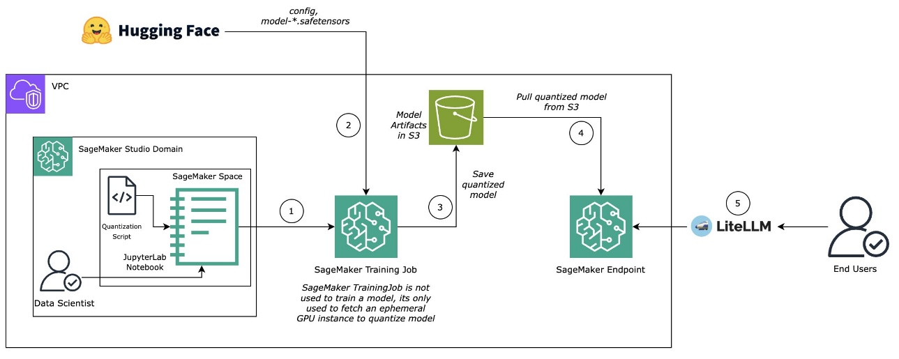
After a model is quantized, it will be saved to Amazon Simple Storage Service (Amazon S3) directly as an output from the SageMaker training job. We’ll uncompress the model and host it as a SageMaker real-time endpoint using a Amazon SageMaker AI large model inference (LMI) container, powered by vLLM. To find the latest images, see AWS Deep Learning Framework Support Policy for LMI containers (see SageMaker section).

...

prebaked_inference_image_uri = f"763104351884.dkr.ecr.{sagemaker.Session().boto_session.region_name}.amazonaws.com/djl-inference:0.33.0-lmi15.0.0-cu128"
...
quant_model = sagemaker.Model(
    image_uri=prebaked_inference_image_uri,
    env={
        "HF_MODEL_ID": f"{remote_upload_s3uri}/", <- Your model S3 path
        "OPTION_MAX_MODEL_LEN": "12000",
        "OPTION_GPU_MEMORY_UTILIZATION": "0.95",
        "OPTION_ENABLE_STREAMING": "false",
        "OPTION_ROLLING_BATCH": "auto",
        "OPTION_MODEL_LOADING_TIMEOUT": "3600",
        "OPTION_PAGED_ATTENTION": "false",
        "OPTION_DTYPE": "fp16",
    },
    role=role,
    name=model_name,
    sagemaker_session=sagemaker.Session()
)
...
pretrained_predictor = quant_model.deploy(
    endpoint_name=endpoint_name,
    initial_instance_count=1,
    instance_type="ml.g5.2xlarge",
    container_startup_health_check_timeout=600,
    wait=False
)
print(f"Your Endpoint: {endpoint_name} is now deployed!")
```

You now have a SageMaker real-time endpoint serving your quantized model and ready for inference. You can query it using the SageMaker Python SDK or litellm, depending on your integration needs.

 from litellm import completion

response = completion(
        model=f"sagemaker/{endpoint_name}", 
        messages=[{ "content": "Hello", "role": "user"}, { "content": "You are a helpful assistant that follows instructions", "role": "system"}],
        temperature=0.1,
        max_tokens=64
    )

Model performance

We will use an ml.g5.2xlarge instance for Llama-3.1-8B and Qwen-2.5-VL-7B models and ml.p4d.24xlarge instance for Llama-3.1-70B model and an LMI container v15 with vLLM backend as a serving framework.

The following is a code snippet from the deployment configuration:

lmi_env = {
    "SERVING_FAIL_FAST": "true",
    "OPTION_ASYNC_MODE": "true",
    "OPTION_ROLLING_BATCH": "disable",
    "OPTION_MAX_MODEL_LEN": "8192",
    "OPTION_TENSOR_PARALLEL_DEGREE": "max",
    "OPTION_ENTRYPOINT": "djl_python.lmi_vllm.vllm_async_service",
}

This performance evaluation’s primary goal is to show the relative performance of model versions on different hardware. The combinations aren’t fully optimized and shouldn’t be viewed as peak model performance on an instance type. Always make sure to test using your data, traffic, and I/O sequence length. The following is performance benchmark script:

#!/bin/bash
export LLM_PERF_CONCURRENT=1
export LLM_PERF_MAX_REQUESTS=$(expr $LLM_PERF_CONCURRENT * 10)
export LLM_PERF_SCRIPT_DIR=$HOME/5_projects/llmperf

export LLM_PERF_OUTPUT=outputs/test-2025-07-08-21-45-57-221

mkdir -p $LLM_PERF_OUTPUT
cp "$0" "${LLM_PERF_OUTPUT}"/

python3 ${LLM_PERF_SCRIPT_DIR}/token_benchmark_ray.py 
    --model "sagemaker/model-2025-07-08-21-01-10-147" 
    --mean-input-tokens 512 
    --stddev-input-tokens 32 
    --mean-output-tokens 256 
    --stddev-output-tokens 16 
    --max-num-completed-requests ${LLM_PERF_MAX_REQUESTS} 
    --timeout 1800 
    --num-concurrent-requests ${LLM_PERF_CONCURRENT} 
    --results-dir "${LLM_PERF_OUTPUT}" 
    --llm-api litellm 
    --additional-sampling-params '{}'

Performance metrics

To understand the impact of PTQ optimization techniques, we focus on five key inference performance metrics—each offering a different lens on system efficiency and user experience:

• GPU memory utilization: Indicates the proportion of total GPU memory actively used during inference. Higher memory utilization suggests more of the model or input data is loaded into GPU memory, which can improve throughput—but excessive usage might lead to memory bottlenecks or out-of-memory errors.
• End-to-end latency: Measures the total time taken from input submission to final output. This is critical for applications where responsiveness is key, such as real-time systems or user-facing interfaces.
• Time to first token (TTFT): Captures the delay between input submission and the generation of the first token. Lower TTFT is especially important for streaming or interactive workloads, where perceived responsiveness matters more than total latency.
• Inter-token latency (ITL): Tracks the average time between successive token outputs. A lower ITL results in smoother, faster-seeming responses, particularly in long-form text generation.
• Throughput: Measures the number of tokens generated per second across all concurrent requests. Higher throughput indicates better system efficiency and scalability, enabling faster processing of large workloads or more simultaneous user sessions.

Together, these metrics provide a holistic view of inference behavior—balancing raw efficiency with real-world usability. In the next sections of this post, we evaluate three candidate models—each varying in size and architecture—to validate inference performance metrics after quantization using AWQ and GPTQ algorithms across different WₓAᵧ strategies. The selected models include:

• Llama-3.1-8B-Instruct: An 8-billion parameter dense decoder-only transformer model optimized for instruction following. Published by Meta, it belongs to the LLaMA (Large Language Model Meta AI) family and is well-suited for general-purpose natural language processing (NLP) tasks.
• Llama-3.3-70B-Instruct: A 70-billion parameter model also from Meta’s LLaMA series, this larger variant offers significantly improved reasoning and factual grounding capabilities, making it ideal for high-performance enterprise use cases.
• Qwen2.5-VL-7B-Instruct: A 7-billion parameter vision-language model developed by Alibaba’s Institute for Intelligent Computing. It supports both text and image inputs, combining a transformer-based text backbone with a visual encoder, making it suitable for multimodal applications.

Note that each model was tested on a different instance type: Llama-3.1-8B on ml.g5.2xlarge, Llama-3.3-70B on ml.p4dn.24xlarge, and Qwen2.5-VL-7B on ml.g6e.4xlarge.

GPU memory utilization

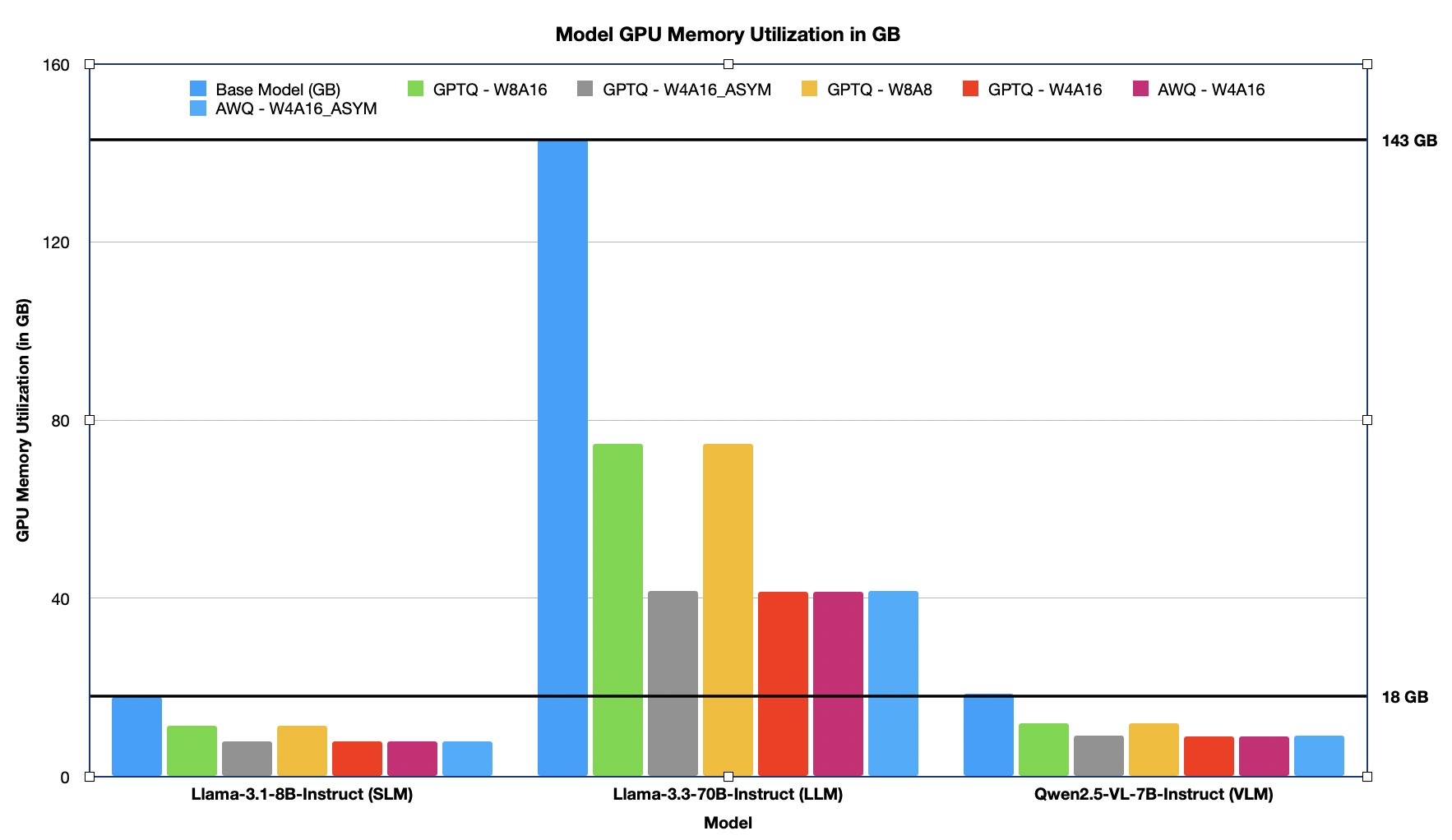
GPU memory utilization reflects how much device memory is consumed during model execution and directly impacts deployability, batch size, and hardware selection. Lower memory usage enables running larger models on smaller GPUs or serving more concurrent requests on the same hardware. Quantization improves compute efficiency and significantly reduces the memory footprint of LLMs. By converting high-precision weights (for example, FP16 or FP32) into lower-bit formats such as INT8 or FP8, both AWQ and GPTQ strategies enable models to consume substantially less GPU memory during inference. This is critical for deploying large models on memory-constrained hardware or increasing batch sizes for higher throughput. In the following table and chart, we list and visualize the GPU memory utilization (in GB) across the models under multiple quantization configurations. The percentage reduction is compared against the base (unquantized) model size, highlighting the memory savings achieved with each WₓAᵧ strategy, which ranges from ~30%–70% less GPU memory utilization after PTQ.

The figure below illustrates the GPU memory footprint (in GB) of the model in its raw (unquantized) form compared to its quantized variants. Quantization results in ~30%–70% reduction in GPU memory consumption, significantly lowering the overall memory footprint.

End-to-end latency

End-to-end latency measures the total time taken from the moment a prompt is received to the delivery of the final output token. It’s a critical metric for evaluating user-perceived responsiveness and overall system performance, especially in real-time or interactive applications.

In the following table, we report end-to-end latency in seconds across varying concurrency levels (C=1 to C=128) for three models of varying size and modality (Llama-3.1-8B, Llama-3.3-70B, and Qwen2.5-VL-7B) under different quantization strategies.

The following graphs showing end to end latency for different concurrency levels for different models.

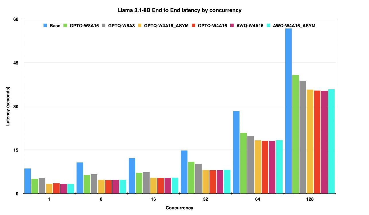
The figure above presents the end-to-end latency of the Llama 3-8B model in its raw (unquantized) form and its quantized variants across concurrency levels ranging from 1 to 128 on the same instance.

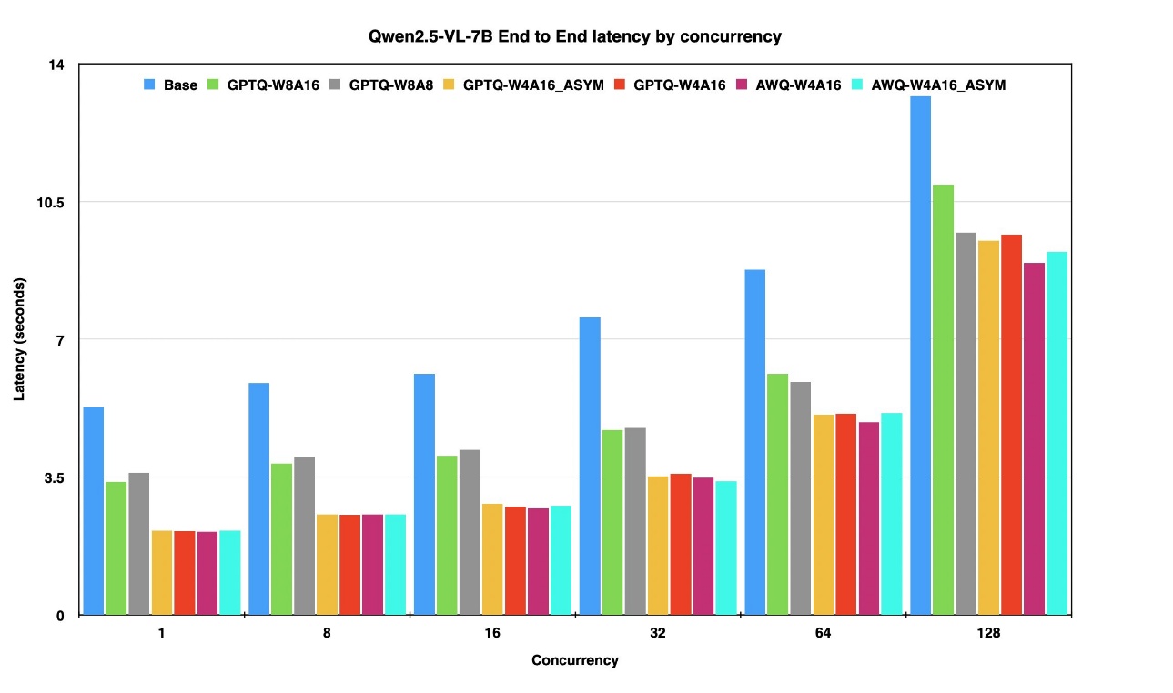
The figure above presents the end-to-end latency of the Qwen 2.7-7B model in its raw (unquantized) form and its quantized variants across concurrency levels ranging from 1 to 128 on the same instance.

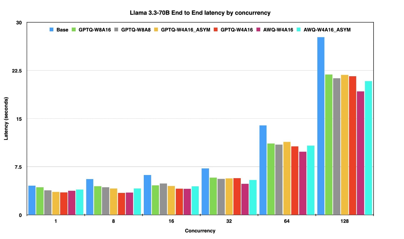
The figure above presents the end-to-end latency of the Llama 3-70B model in its raw (unquantized) form and its quantized variants across concurrency levels ranging from 1 to 128 on the same instance.

Time to first token

TTFT measures the delay between prompt submission and the generation of the first token. This metric plays a crucial role in shaping perceived responsiveness—especially in chat-based, streaming, or interactive applications where initial feedback time is critical. In the following table, we compare TTFT in seconds for three models of varying size and modality—Llama-3.1-8B, Llama-3.3-70B, and Qwen2.5-VL-7B—under different quantization strategies. As concurrency increases (from C=1 to C=128), the results highlight how quantization techniques like AWQ and GPTQ help maintain low startup latency, ensuring a smoother and faster experience even under high load.

Inter-token latency

ITL measures the average time delay between the generation of successive tokens. It directly affects the smoothness and speed of streamed outputs—particularly important in applications involving long-form text generation or voice synthesis, where delays between words or sentences can degrade user experience. In the following table, we analyze ITL in seconds across three models of varying size and modality—Llama-3.1-8B, Llama-3.3-70B, and Qwen2.5-VL-7B—under different quantization schemes. As concurrency scales up, the results illustrate how quantization strategies like AWQ and GPTQ help maintain low per-token latency, ensuring fluid generation even under high parallel loads.

Throughput

Throughput measures the number of tokens generated per second and is a key indicator of how efficiently a model can scale under load. Higher throughput directly enables faster batch processing and supports more concurrent user sessions. In the following table, we present throughput results for Llama-3.1-8B, Llama-3.3-70B, and Qwen2.5-VL-7B across varying concurrency levels and quantization strategies. Quantized models maintain—and in many cases improve—throughput, thanks to reduced memory bandwidth and compute requirements. The substantial memory savings from quantization allows multiple model workers to be deployed on a single GPU, particularly on high-memory instances. This multi-worker setup further amplifies total system throughput at higher concurrency levels, making quantization a highly effective strategy for maximizing utilization in production environments.

Conclusion

Post-training quantization (PTQ) techniques like AWQ and GPTQ have proven to be effective solutions for deploying foundation models in production environments. Our comprehensive testing across different model sizes and architectures demonstrates that PTQ significantly reduces GPU memory utilization. The benefits are evident across all key metrics, with quantized models showing better throughput and reduced latency in inference time, including high-concurrency scenarios. These improvements translate to reduced infrastructure costs, improved user experience through faster response times, and the flexibility of deploying larger models on resource-constrained hardware. As language models continue to grow in scale and complexity, PTQ offers a reliable approach for balancing performance requirements with infrastructure constraints, providing a clear path to efficient, cost-effective AI deployment.

In this post, we demonstrated how to streamline LLM quantization using Amazon SageMaker AI and the llm-compressor module. The process of converting a full-precision model to its quantized variant requires just a few simple steps, making it accessible and scalable for production deployments. By using the managed infrastructure of Amazon SageMaker AI, organizations can seamlessly implement and serve quantized models for real-time inference, simplifying the journey from development to production. To explore these quantization techniques further, refer to our GitHub repository.

Special thanks to everyone who contributed to this article: Giuseppe Zappia, Dan Ferguson, Frank McQuillan and Kareem Syed-Mohammed.

About the authors

Pranav Murthy is a Senior Generative AI Data Scientist at AWS, specializing in helping organizations innovate with Generative AI, Deep Learning, and Machine Learning on Amazon SageMaker AI. Over the past 10+ years, he has developed and scaled advanced computer vision (CV) and natural language processing (NLP) models to tackle high-impact problems—from optimizing global supply chains to enabling real-time video analytics and multilingual search. When he’s not building AI solutions, Pranav enjoys playing strategic games like chess, traveling to discover new cultures, and mentoring aspiring AI practitioners. You can find Pranav on LinkedIn

Dmitry Soldatkin is a Senior AI/ML Solutions Architect at Amazon Web Services (AWS), helping customers design and build AI/ML solutions. Dmitry’s work covers a wide range of ML use cases, with a primary interest in Generative AI, deep learning, and scaling ML across the enterprise. He has helped companies in many industries, including insurance, financial services, utilities, and telecommunications. You can connect with Dmitry on LinkedIn.